Room Correction using Biquad Filters

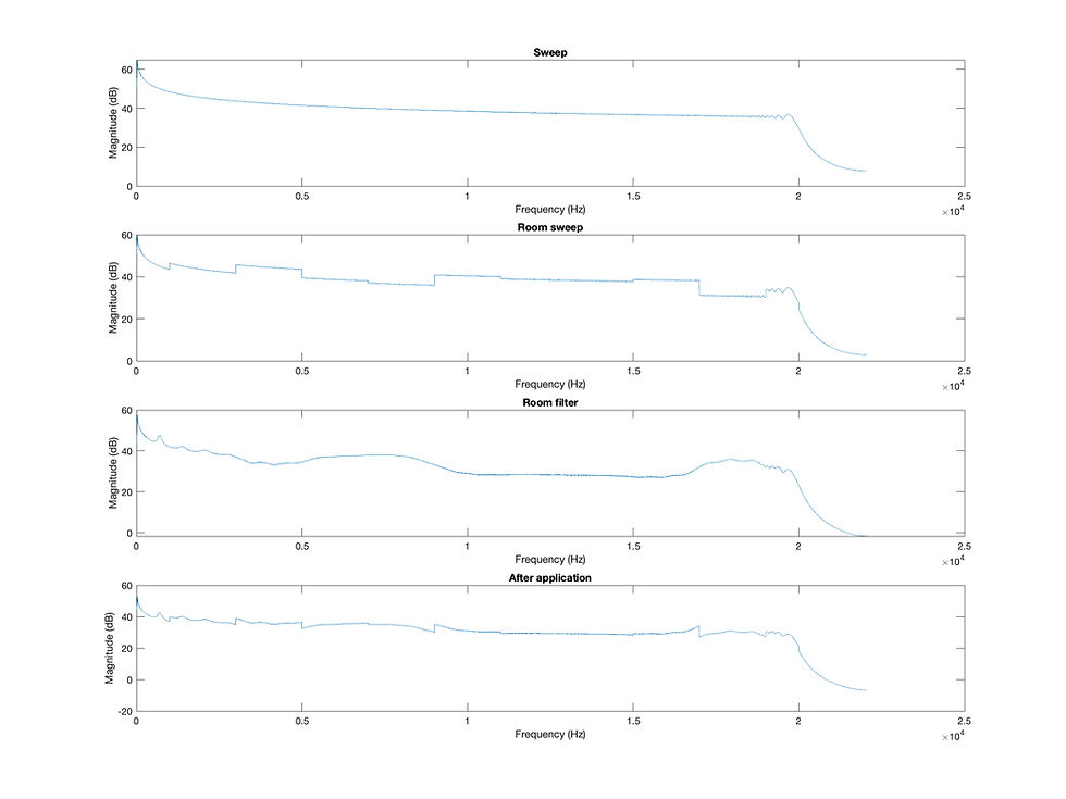
Gain randomly ranged from -5 to 5, Q = 6:

One of the functionalities I wanted my speakers to have is room correction. It has become such a standard/normal function that it seems to be the equivalent of the "seat belt" or the "air bag" of a car—or perhaps, that would be Dolby Atmos.

Here is a relatively simple method of implementing room correction using biquad filters that I came up with one Friday night—my use of free time typically consists of staring at Matlab, watching The Office, and building my speakers.

First, we construct a signal in Matlab. This would be an exponential sine sweep since we will be using it to get the room's frequency response.

f_start = 20;
f_end = 20000;
T = 1;
fs = 44100;
t = linspace(0, T, fs * T);
k = T / log(f_end / f_start);
f_t = f_start * exp(t / k);
sweep = sin(2  pi  f_start  k  (exp(t / k) - 1));

It is important to note that we are not using buffers for the FFT, although real life applications will be using buffers. This is simply to verify that the logic behind the program works as intended. To counter the inaccuracies from using a single FFT, we make the timing of the sweep incredibly short.

The next step would be to normalize the sweep, and get the magnitude response from the frequency response using FFT.

sweep = sweep / max(abs(sweep));
N = length(sweep);                    
sweep_fft = fft(sweep);                
sweep_fft = sweep_fft(1:N/2+1);          
%sound(sweep, fs);
magnitude = abs(sweep_fft);

Next, in order to simulate a room's frequency response, we alter the original magnitude response by doing ".*" to the original FFT. Here are some frequency bands that are 2000Hz apart from each other. Their gain levels are determined randomly by "randi", and range from -10 to 10 dB.

gain_db = zeros(1, N/2+1);
gain_db(f >= 20 & f < 1000) = randi([-10, 10], 1);
gain_db(f >= 1000 & f < 3000) = randi([-10, 10], 1);
gain_db(f >= 3000 & f < 5000) = randi([-10, 10], 1);
gain_db(f >= 5000 & f < 7000) = randi([-10, 10], 1);
gain_db(f >= 7000 & f < 9000) = randi([-10, 10], 1);
gain_db(f >= 9000 & f < 11000) = randi([-10, 10], 1);
gain_db(f >= 11000 & f < 13000) = randi([-10, 10], 1);
gain_db(f >= 13000 & f < 15000) = randi([-10, 10], 1);
gain_db(f >= 15000 & f < 17000) = randi([-10, 10], 1);
gain_db(f >= 17000 & f < 190000) = randi([-10, 10], 1);
gain_db(f >= 19000 & f < 20000) = randi([-10, 10], 1); 
gain_linear = 10.^(gain_db / 20);
sweep_fft(1:N/2+1) = sweep_fft(1:N/2+1) .* gain_linear; 
roomsweep = ifft(sweep_fft(1:N/2 + 1));
roommagnitude = abs(sweep_fft);

After converting the gain levels from dB to linear scale, we apply the gain to the original signal, and take the absolute value of the FFT to get the room's magnitude response.

To create the filters for correcting the room's response, we first need to decide on how many filters we would like to implement. This number is determined by "numBands". Naturally, the more filters there are, the more precise the correction will be. For this example, we set the bandwidth to be the unfortunate 666, which means there will be 30 peaking filters. The Q-value can be predetermined by trial and error. Too small of a Q-value can result in unpredictable responses.

f0 can be determined by using linspace. Create a copy of the original sweep signal to reiterate through a loop.

numBands = round((f_end-f_start)/666);
Q = 8;
f0_array = round(linspace(f_start, f_end, numBands));
filteredSignal = sweep;
for k = 1:numBands
    f0 = f0_array(k);  
    if f0 == 20 || f0 == 20000
        continue;
    end
    sumsweep = 0;
    sumroom = 0;
    for n = (round(f0-349.5)):(round(f0+349.5))
        sumsweep = sumsweep + magnitude(n);
        sumroom = sumroom + roommagnitude(n);
    end
    sumsweeprms = rms(sumsweep);
    sumroomrms = rms(sumroom);
    meansweepdb = mag2db(sumsweeprms); 
    roomgaindB = mag2db(sumroomrms);
    gaindB = roomgaindB - meansweepdb;
    gainlinear = db2mag(-gaindB);

    w = 2 * pi * (f0 / fs);
    alpha = sin(w) / (2 * Q);
    b0 = 1 + gainlinear * alpha;
    b1 = -2 * cos(w);
    b2 = 1 - gainlinear * alpha;
    a0 = 1 + alpha;
    a1 = -2 * cos(w);
    a2 = 1 - alpha;

    b = [b0/a0, b1/a0, b2/a0];
    a = [a0/a0, a1/a0, a2/a0];

    filteredSignal = filter(b, a, filteredSignal);
end

We skip f0 = 20 and f0 = 20000 since the bandwidths of both will go out of bound. To find how much gain we need to cut/boost, we first find the sum of magnitudes at each frequency from the original response and room's reponse. This is achieved by a loop that iterates through half the bandwidth on the left and right side of f0. The sums are then converted to their rms values. I chose rms values so that the peak value of a particular band does not incorrectly influence the difference too much.

Now that we have the rms magnitudes of each frequency band, we can convert them into dB, calculate the difference, and convert them back to linear scale for filter use. The gain is negative so that it can be used for correction.

And finally we can calculate the coefficients for the filter.

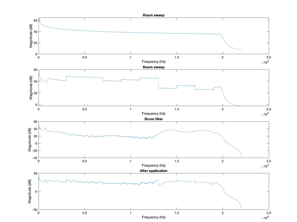
Finally, to plot filter magnitude, we can do what we did for the original sweep.

filteredSignal = filteredSignal / max(abs(filteredSignal));
filteredSignal_fft = fft(filteredSignal);
filteredSignal_fft = filteredSignal_fft(1:N/2+1);
filterMagnitude = abs(filteredSignal_fft);
finalMag = (filterMagnitude .* roommagnitude)./magnitude;

figure;
subplot(4, 1, 1);
plot(f, 20*log10(magnitude));
xlabel('Frequency (Hz)');
ylabel('Magnitude (dB)');
title('Sweep');

subplot(4, 1, 2);
plot(f, 20*log10(roommagnitude));
xlabel('Frequency (Hz)');
ylabel('Magnitude (dB)');
title('Room sweep');

subplot(4, 1, 3);
plot(f, 20*log10(filterMagnitude));
xlabel('Frequency (Hz)');
ylabel('Magnitude (dB)');
title('Room filter');

subplot(4, 1, 4);
plot(f, 20*log10(finalMag));
xlabel('Frequency (Hz)');
ylabel('Magnitude (dB)');
title('After application');

Gain randomly ranged from -10 to 10, Q = 8: